CBC latches, CPU consumption, and wait time

This page has been permanently moved. Please CLICK HERE to be redirected.

Thanks, Craig.

What's this about?

When a system is experiencing severe cache buffer chain (CBC) latch contention and many of the child latches are active, one of the common Oracle focused solutions is to increase the number of CBC latches. This typically yields some benefit because both the CPU time and the non-idle wait time per SQL statement execution decreases. But why is CPU time and non-idle wait time reduced? This is what this blog entry is all about...

If you just want the "bottom line," scroll down to the last section.

Getting a time perspective.

For the experimental results to really make sense, we need to look at performance from a time and also a unit of work time perspective.

One way to categorize the time related to processing a piece of Oracle work (e.g., buffer get, SQL statement) is to place the time into two buckets; CPU time and non-idle Oracle wait time (i.e., wait time). For example, if on average a SQL statement consumes 1 second of CPU time and 2 seconds of wait time per execution, then the elapsed time is 3 seconds.

For reference, a buffer get is sometimes call a logical IO or for short LIO or lio. This statistic can be gathered from v$sesstat and v$sysstat with the statistic name session logical reads.

It turns out that the CPU consumption per piece of Oracle work is very consistent regardless of the workload intensity. (This is a key subject in my Oracle performance courses and I will not get into the details in this blog entry.) What continues to slow performance is as the workload intensity increases the wait time increases.

So it follows that there are three fundamental ways to reduce the time it takes to process a buffer get, SQL statement, or a group SQL statements. You can either reduce the amount of work required (i.e., workload intensity), the CPU consumption, or the non-idle Oracle wait time. Increasing parallelism is also another option, but I'll save that discussion for another time.

When we talk about time, it needs to be related to a task. Like the time related to driving to work, mowing the lawn, having a conversation with someone, or completing a SQL statement. These tasks are actually made up of many small movements or pieces of work. When referring to driving to work, a movement that makes practical sense can be the number tire revolutions. When referring to a SQL statement, a practical movement could be a buffer get. I commonly call a movement a unit of work or a piece of work.

Let's focus on a buffer get as the movement, that is a unit of work. The elapsed time of a SQL statement can be expressed as the sum of the time for doing all the necessary buffer gets, that is, all the movements as expressed as buffer gets. For example, if a SQL statement's elapsed time is 3 seconds and 10000 buffer gets are required to complete the statement, then the average time to complete each buffer get is 0.0003 seconds or simply 0.0003 seconds per buffer get.

One of the advantages of working at the unit of work level is we can take advantage of all the research, theory, and mathematics related to Operations Research. In my next blog entry, I will demonstrate how this blog's experimental results match Operations Research.

As mentioned above, there are three fundamental ways to reduce the time it takes to process a piece of work, that is, a unit of work. We can reduce the CPU it takes to process the piece of work, reduce the wait time related to the piece of work, or we can reduce the number of pieces of work we must process. For example, suppose a SQL statement's elapsed time is 3 seconds, 10000 buffer gets are required to complete the statement, 2 seconds of CPU are consumed, and there is 1 second of Oracle non-idle wait time. With just these bits of information we know, can generalize, and can quantify the performance situation like this:

• 10000 buffers were processed over the 3 second elapsed time. This means the workload was 3333.333 buffers/second or 3.333 buffers/ms. (10000/3 buffers/sec X 1/1000 sec/ms = 3.333 buffers/ms)
• It took 2 seconds of CPU to process all 10000 buffers. This means the CPU time required to process a single buffer was 0.0002 seconds or 0.0002 sec/buffer or 0.020 ms/buffer. (2/10000 seconds/buffer X 1000/1 ms/sec = 0.200 ms/buffer)
• There was 1 second of non-idle Oracle wait time involved when processing the 10000 buffers. This means the wait time associated with processing each buffer was 0.0001 seconds or 0.0001 sec/buffer or 0.100 ms/buffer. (1/10000 seconds/buffer X 1000/1 ms/sec = 0.100 ms/buffer)

Therefore, if we can reduce the workload, the CPU time, or the wait time then the elapsed time will likely be reduced. To reduce the words, let's create an equation.

E = Work X Time per Work

where:

E is the elapsed time (e.g., 2 seconds)
W is the amount of work to be completed (e.g., 10000 buffer gets)
Time per Work is the CPU and the wait time associated with processing a single piece of work. (e.g., 3 seconds.

Taking this a step further:

E = Work X ( CPU time per work + wait time per work )

And there we have it! We can reduce the elapsed time (E) by either reducing the work (Work), the CPU time per unit of work, or by reducing the wait time per unit of work. While this may seem rather theoretical (and it is to some degree), as I will detail below this is important to understanding why adding CBC latches to a system that is experiencing severe CBC latch contention can improve performance.

A warning: While this a very simple way to model elapsed time and valid in many cases, it is also limited...much like a paper airplane models a commercial jet or a benchmark models a real production Oracle system. But just as with many models, we can learn a tremendous amount about a specific area of interest in a very complicated system...that for practical purposes is impossible to replicate.

How does this relate to adding CBC latches?

Note: This is probably the most important section in this blog, so please read it carefully.

Answer: Because when we add CBC latches, Oracle does not have to spin as many times and/or sleep as many times when acquiring a latch. Spinning on a latch consumes CPU, therefore reducing spinning reduces CPU consumption, which reduce CPU consumption per unit of work. Sleeping less often reduces non-Oracle wait time (latch: cache buffer chains), which reduces wait time per unit of work. Said another way, when we spin less, we consume less CPU. And when we sleep less, we wait less.

Another way of looking at this is to understand that when a process spins, it is actually executing lines of Oracle code. For example, suppose each spin executes 5 lines of code and to process a buffer it is currently taking around 4000 spins. However, through Oracle tuning it is now only taking 100 spins to process a buffer. This means the lines of code executed went from 20000 (5 X 4000) down to 500 (5 X 100). Since each line of code executed consumes CPU, we have purposefully and truly reduced the CPU required to process a buffer get and consequently also a buffer get dependent SQL statement's elapsed time. But it gets better! If a process spins less they are more likely to sleep less also, reducing wait time.

From a conceptual perspective, think of it like this: If there are more latches available yet the number of sessions competing for the latches remains the same, a session will be competing with fewer sessions when attempting to acquire the latch. In addition to this, a session is less likely to be asking for a latch that another process already has acquired. This results in less spinning (CPU reduction) and sleeping (wait time reduction).

But is this what really happens in Oracle systems?

Short answer: Yes. To demonstrate this an experiment is needed.

Experimental Design.

I created a system with a severe cache buffer chain load. The workload consisted of many queries in which all the blocks reside in the buffer cache. The server consists of a single 4 core Intel CPU, running Red Hat Linux, and Oracle 11.2.

I actually did two experiments. They are related but with one key difference. One only alters the number of CBC latches (Experiment 1) and the second alters both the CBC latches and the number of chains (Experiment 2).

The Downloads.

Here are the download links:

• Click here, to download and view online the text file containing the various data collection and reporting scripts.
• Click here, to download and view online the PDF file of the Mathematica notebook for Experiment 1.
• Click here, to download and view online the PDF file of the Mathematica notebook for Experiment 2.
• Click here, to download the source Mathematica file for Experiment 1.
• Click here, to download the source Mathematica file for Experiment 2.
• Click here, to download all the above five file in a single zip file.

Experimental Design - Experiment 1: Altering the CBC latches

The workload consisted of 20 processes running queries in which all the blocks reside in the buffer cache. This created a massive CPU bottleneck with an OS CPU run queue consistently between 12 and 20 with the CPU utilization pegged at 100%.

I was disappointed I could not simply reduce the number of CBC latches to as low as I wanted. This would allow a very nice trend to develop...but Oracle is not interested in my experiments...they want to ensure a DBA does not make a CBC change that will clearly, as we'll see, hurt performance.

For this experiment I altered the number of CBC latches (parameter, _db_block_hash_latches); 1024 (minimum Oracle would allow), 2048, 4096, 8192, 16384, and 32768. For each CBC latch setting I gathered 90 samples at 180 seconds each. This means 540 samples were gathered for a total of 97,200 seconds...but this does not include the instance restart time, stabilization time, etc. ...I gathered lots of samples!

Experimental Design - Experiment 2: Altering both CBC latches and Cache Buffer Chains

The workload consisted of 12 processes running queries in which all the blocks reside in the buffer cache. This created a massive CPU bottleneck with an OS CPU run queue consistently between 5 and 12 with the CPU utilization hovering around 94% to 99%. The bottleneck intensity was not nearly as severe as in Experiment 1 and probably more realistic then the Experiment 1 bottleneck.

By setting the number of cache buffer chains below 1024 (parameter, _db_block_hash_buckets), I was also able to set the number of CBC latches below 1024 (parameter, _db_block_hash_latches). It turns out that Oracle will respect the number of chain settings (although it will round up to the next power of two) and then allow me to set the number of CBC latches to the number of chains. For example, if I set the number of chains and latches to 100, when the instance is restarted the actual number of chains and latches will be 256. And if I set the number of chains and latches to 300, when the instance is restarted the actual number of chains and latches will be 512.

For this experiment I altered the number of CBC latches and chains to; 256, 512, 1024, 2048, 4096, 8192, 16384, 32768, and 65536. For each CBC latch setting I gathered 60 samples at 180 seconds each. Which means 540 samples were gathered for a total of 97,200 seconds...but this does not include the instance restart time, stabilization time, etc. ...again, I gathered lots of samples.

Experimental Results Summary - Experiment 1

With each increase in the number of latches, both the CPU and wait time per buffer get decreased. (The decrease is statistically significant with an alpha of 0.05.) While the CPU time per buffer get decreased around 4%, the wait time decreased from 19% to 55% resulting in a total time per buffer get decrease from 11% to 28%.

To keep things simple and to the point, I only included four figures below. You can view/download the entire statistical analysis, which contains around 30 graphs and all data samples by clicking on the "view PDF for Experiment 1" link in The Downloads section above. Here are the details...

Figure 1.

Figure 1 above is a statistical summary for the experimental results. Here is a quick description of the columns.

• CBC latches is the number of latches during the sample gathering.
• Avg L is the average number of buffer gets processed per millisecond. L stands for Lambda, which is the common symbol for the arrival rate.
• Avg St is the average CPU consumed per buffer get processed. This is also called the service time, hence St. This is calculated as the total number CPU consumed divided by the total number of buffer gets during the sample interval of 180 seconds.
• Avg Qt is the average non-idle wait time per buffer get. This is also called the queue time, hence Qt. This is calculated as the total non-idle wait time divided by the total number of buffer gets during the sample interval of 180 seconds.
• Avg Rt is the time to process a single buffer get. This is also called the response time, hence Rt. It is calculated as simply the service time plus the queue time, that is, the CPU time plus the non-idle wait time per buffer get.

Figure 2.

Figure 2 above shows the CPU time (blue line) and the wait time added to that (red-like line) per buffer get versus the number of latches. While there is an initial drop in the CPU time per buffer get, the only significant decrease occurs when going from 1024 latches to 2048 latches. In this experimental system, Oracle was not able to achieve additional efficiencies by increasing the number of CBC latches. As I mentioned above, during the entire experiment the average CPU utilization was 100% and the run queue was usually well above 12.... which is over 3X the number of CPU cores!

Figure 3 below is a response time graph based on our experimental data (shown in Figure 1 above) integrated with queuing theory. The three plotted points are based entirely on our sample data's arrival rate (buffer get per ms, column Avg L) and response time (CPU time and wait time ms per buffer get, column Avg Rt) for 1024 latches (blue point), 2048 latches (red point), and 4096 latches (orange point). When we integrate key Oracle performance metrics with queuing theory, we can create the classic response time curve, which is what you see in Figure 3 below. (This is one of the topics, including constructing the below graph, we delve into in my Advanced Oracle Performance Analysis course. This is also introduced in the last chapter of my book, Oracle Performance Firefighting.

In contrast to the typical "big bar" graph which shows total time over an interval or snapshot, the response time graph shows the time related to complete a single unit of work. In our case, the single unit of work is a single buffer get. The response time is the sum of both the CPU time and the wait time to process a single buffer get.

Figure 3.

Notice that the CPU time per buffer get only significantly drops from the blue line to the red line. This is easier to see when looking at the flat lines near the left of the graph and when zooming into the graph. The much larger response time drop occurs because the wait time per buffer get decreases. Therefore, based on our experimental data, a small decrease in CPU per buffer get results into much larger decrease in the wait time and also the resulting response time. While the details are out of scope for this blog entry, queuing theory states that when the CPU per unit of work decreases, the response time curve drops and shifts to the right... and this is exactly what we see in Figure 3!

Also, notice that the blue dot is further to the left then both the red and orange dots. If the workload did not increase when the number of latches was increased, the response time improvement would have been much more dramatic. However, the system was allowed to stabilize and in this case, more worked flowed through the system. This workload increase diminishes the response time improvement... which probably makes the business very happy and possible the users as they "get more work done."

Figure 4.

Figure 4 above is simply a histogram containing the response times for all 90 samples for each latch sample sets (1024, 2048, etc.). The far left histogram is related to 32768 latches and the far right histogram is related to 1024 latches. While sample set five (16384 latches, counting right to left) does not look that different from sample set four (8192 latches), statistically there is a difference. And as you might expect then, there is a statistically significant difference between each sample sets CPU time plus wait time per buffer get. If you really want to dig into the statistics, which is actually pretty cool for this experiment, click on the "view PDF for Experiment 1" link in The Downloads section above

Experimental Results Summary - Experiment 2

With each increase in the number of cache buffer latches and chains, all but the final test comparing 32656 and 65536 latches (and chains) clearly show both the CPU and wait time per buffer get decreased. (The decrease is statistically significant with an alpha of 0.05.) And the decrease is dramatic. Especially when the number of chains and latches are relatively low.

For me, Experiment 2 is more dramatic (and more personally satisfying) then Experiment 1. The experimental setup is also different. First, I reduced the number of load processes from 20 to 12. While there was still a severe and clear CPU bottleneck and intense CBC latch contention, it wasn't nearly as ridiculously intense as in Experiment 1. Second, I was also able to reduce the number of CBC latches down to 256. This allows us to see the impact of adding latches when there are initially relatively few.

Why the number of cache buffer (CB) chains is related to performance.

It's actually pretty simple. The cache buffer chain structure is accessed to determine if a block exists in the buffer cache. Therefore, each block cached in the buffer cache must be represented in the cache buffer chain structure. Oracle chose a hashing algorithm and associated memory structure to enable extremely consistent fast searches (usually). To drastically simplify, the hashing structure includes a number of chains. Since the number of buffers in the buffer cache is constant (let's forget about Oracle's ability to dynamically resize the buffer cache...) as the number of chains increase, then the chain length decreases (on average). Therefore, one way to increase the chain length and also increase search time (bad for performance) is to decrease the number of chains. Of course you would never do this in a production system, without a very, very good reason.

And it follows that increasing the number of chains will decrease search time, because the average chain length will be shorter. This is true and Oracle Corporation knows it. So much so, the default number of chains is greater than the number of buffers, resulting in an average chain length of less than one. However, if we severely limit the number of CB chains causing longer chains and concurrency issues, like I have done in this experiment, as the number of chains is increased we should see a significant performance improvement.

Additionally, keeping one CBC latch per chain ensures processes will not be competing for different chains protected by the same CBC latch! This is called false contention.

If you would like to visually see how the CBC structure works and also the buffer cache in general, I have created a free interactive visual tool you can experiment with. You can download it here. It's pretty cool! I also blogged about the initial release (think of this as the user guide) here.

Now let's go a little deeper and relate the experimental results with the architecture and memory structures.

To keep things simple and to the point, I only included four figures plus two others for those who want a little more detail. You can view/download the entire statistical analysis, which contains well over 30 graphs and all data samples clicking on the "view PDF for Experiment 2" link in The Downloads section above.

Figure 5.

Figure 5 above is a statistical summary for the experimental results. Figure 5 clearly shows that with each increase (except the last) in CB chains and latches, both the CPU time and wait time per buffer get decrease. However, it is also equally obvious the improvement diminishes as the number of CB chains and latches increase. On my experimental system, the performance improvement while statistically significant, pretty much becomes a non-issue once there are 4096 CB latches and chains. Interestingly, with the 1.5GB buffer cache I used, without my specifically setting the number of CBC latches and chains, Oracle automatically created 8192 CBC latches and 262144 CB chains. Not bad!

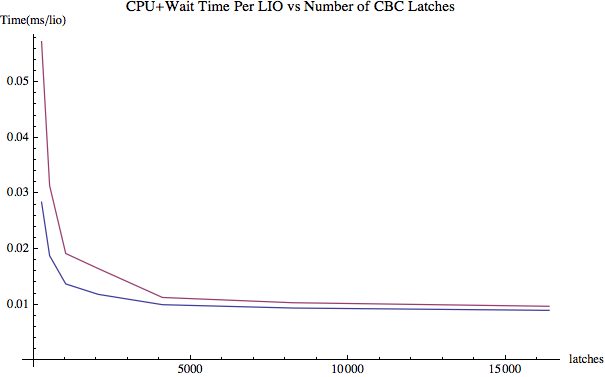
Figure 6.

Figure 6 above shows the CPU time (blue line) and the wait time added to that (red-like line) per buffer get versus the number of latches; this is the response time per buffer get. I did not include the last two sample sets because it diminishes our view of the key area of the graph (far left). There was a dramatic drop in both CPU consumption and wait time per buffer get (i.e., response time) going from 256, 512, and to 1024 latches and buckets. But then the benefit quickly diminishes, yet still significant until we have more than 4096 latches and buckets.

In this experimental system, Oracle was clearly able to achieve additional efficiencies by increasing the number of CBC latches up to 4096 latches and buckets.

Figure 7 below is a response time graph based on our experimental data (Figure 5) and queuing theory. I explained this graph in some detail above related to Figure 3. In Experiment 2, the blue line is based our 256 latches and chains data, the red line on our 512 latches and chains data, and the orange line is based on 1024 latch and chain data. The results are similar to Experiment 1 in pattern, but the drop in the CPU time per buffer get, the drop in the wait time per buffer get and the resulting workload when the system stabilized is much more dramatic. I suspect this is due to the fact that the initial number of latches was significantly lower (256 compared to 1024), the number of chains was significantly lower (256 compared to probably over 100,000), and the load was not so ridiculously intense as in Experiment 1.

Figure 7.

Looking closely at Figure 7 above, notice that for each increase in latches and buckets (going from the blue, red, to orange lines) while the CPU consumption and wait time per buffer get (i.e., response time) continued to decrease (the plotted point) while the arrival rate (i.e., the workload and labeled Avg L in Figure 5) continued to increase. This means the system was able to process more work AND process it faster! From my years of consulting, this is very characteristic of what happens in real production systems.

Figure 8.

Figure 8 above is simply a histogram containing all 90 samples for each of the nine latch sample sets (going right to left: 256, 512, 1024, 2048, 4096, 8192, 16384, 32768, and 65536). You can easily see the dramatic difference in response time and their diminishment as the number of latches and chains increases! All the final response time set (65536 latches and chains) differed significantly from the previous lower latch setting. (details below)

If you really want to dig into the statistics, which is actually pretty cool for this experiment, click on the "view PDF for Experiment 2" link in The Downloads section above.

Significance Details (for those who can't get enough)

If you are fascinated with statistical significance testing or just plain confused about how a P-Value relates to reality, take a look at the two figures below; Figure 9 and Figure 10. For background, if two sample sets match exactly (basically comparing a sample set to itself) and a significance test is performed, the resulting P-Value will be 1.0. If the P-Value is less than 0.05 (a standard threshold or cutoff value) then we will say there is a statistically significant difference between our sample sets. Also, while many of the sample sets were not normally distributed, the response times for sample set 7, 8, and 9 (16384, 32768, and 65536 latches and chains respectively) are indeed normally distributed. Mathematica automatically chose the T test for the significant test (specially what it calls, K-Sample T).

Figure 9.                      Figure 10.

Both Figure 9 and Figure 10 are smoothed histograms of different sample sets based on the experimental data's CPU time plus wait time per buffer get, that is, the response time (ms/lio). The difference between the two figures is Figure 9 is based on the response time samples from sample set 7 and 8 (16384 and 32657 CBC latches and chains) and in contrast, Figure 10 is based on the response time samples from sample set 8 and 9 (32657 and 65536 CBC latches and chains). We can visually see there is a clear difference between sample set 7 and 8 (Figure 9) but there does not appear to be a difference between sample set 8 and 9 (Figure 10). But visual analysis alone can bring us to an incorrect conclusion.

In our two cases, the visual comparison leads us to the correct conclusion because the P-Value comparing sample set 7 and 8 (Figure 9) is 0.0000 whereas the P-Value comparing sample set 8 and 9 (Figure 10) is .64605.  The P-Value for Figure 9 clearly is below our 0.05 cut off and is therefore our sample sets are deemed different. However, the P-Value for Figure 10 is clearly above our 0.05 cut off and therefore statistically there is no real difference between sample set 8 and 9. If you look closely at Figure 5, Figure 6, Figure7, and Figure 8 above we can also infer this, but doing the actual significance test is always better... especially if you're going to stand up in front of management and make a statement.

Just "Give me the facts!" summary...bottom line

1. A CPU bottlenecked CBC constrained Oracle system's performance will likely be improved by increasing the number of CBC latches beyond Oracle's default values... up to a point.

The bottom line for my experimental system is this: With a clear and very intense CPU bottleneck along with severe CBC latch contention, the CPU time and non-idle wait time per buffer get decreased as the number of CBC latches increased and also as the number of CB latches and chains increased... up to a point.

The bottom line for any Oracle system is this: With a clear and very intense CPU bottleneck along with severe CBC latch contention, the CPU time and non-idle wait time per buffer get decreased as the number of CBC latches was increased beyond the Oracle default value. But the benefit diminished as the number of CBC latches continued to increase. This statement is based on my experiments and field observations and is in no way a performance guarantee.

2. Performance improves because when we add CBC latches, Oracle does not have to spin as many times (CPU consumption reduced) and/or sleep as many times (wait time reduced) when acquiring a CBC latch.

3. If a SQL statement is constrained by CBC latch contention and buffer gets, as the time to process buffer get decreases then so will the SQL statement elapsed time.

4. Oracle tuning is required for optimal performance.

This experiment should reaffirm that tuning Oracle can make a significant performance difference. Of course tuning SQL, running SQL less often, and increasing OS capacity can increase performance. But if you want optimal performance, with very little effort in this case I would argue, you need to be able to tune Oracle as well.

I hope you enjoyed this blog entry as much as I did when creating it!

Thanks for reading,

Craig.



If you enjoyed this blog entry, I suspect you'll get a lot out of my courses; Oracle Performance Firefighting and Advanced Oracle Performance Analysis. I teach these classes around the world multiple times each year. For the latest schedule, click here. I also offer on-site training and consulting services.

P.S. If you want me to respond with a comment or you have a question, please feel free to email me directly at craig@orapub .com. I use a challenge-response spam blocker, so you'll need to open the challenge email and click on the link or I will not receive your email. Another option is to send an email to OraPub's general email address, which is currently orapub.general@gmail .com.